Quantum Computing, Beyond Qubits – Part 1: Starting With the Basics

1. Overview

In 1996, Peter Shor published his paper on Polynomial-Time Algorithms for Prime Factorization and Discrete Logarithms on a Quantum Computer. At that instant, the topic of quantum computing suddenly rose to a whole new level.

The paper received a lot of interest from the community as prime factorization of large numbers was considered extremely difficult and was therefore used as the basis for RSA cryptography.

At that time, however, no quantum computers existed, at least not in the sense that we are familiar with.

It wasn’t until 1998 that a physical quantum computing machine could be demonstrated.

That system was a 2-qubit quantum computer successfully used to demonstrate the Deutsch-Jozsa algorithm.

The Deutsch-Jozsa problem had very little practical use; its sole purpose is to provide an example of a problem that is easy to solve on a quantum computer but difficult to solve on a classical one.

Today, Google and IBM race towards quantum supremacy, a term coined by John Preskill, which refers to achieving practical computational capabilities impossible on classical computers.

The below text is from IBM’s Q System One website; it shows how far quantum computing has travelled in the last couple of years:

In 2016 we were the first company to put quantum computing on the cloud and into the hands of hundreds of thousands of users. Today, anyone can access an expanded selection of quantum cloud services based on IBM Quantum System One technology to research and explore new problems on our systems.

But what is quantum computing? Can we determine how fast it is compared to classical machines?

In this article, we will use David Deutsch’s algorithm as our background to try and answer the following questions:

How quantum computing works
How quantum computers differ from their classical counterparts
How a difficult problem can be solved efficiently using quantum computing

But before we proceed, a word of caution.

3. How Quantum Computing Works

3.1 Bits vs Qubits

One of the first results in the mathematics of computation […] was the distinction between computable and non-computable functions[…]. Central to this result is Church’s thesis, which says that all computing devices can be simulated by a Turing machine. This thesis greatly simplifies the study of computation, since it reduces the potential field of study from any of an infinite number of potential computing devices to Turing machines.

— Peter Shor – Polynomial-Time Algorithms for Prime Factorization and Discrete Logarithms on a Quantum Computer, 1996

As you probably may know, a classical computer manipulates “bits” of data. A bit is a discrete unit of information allowing you to answer a question with a Yes or a No. A series of n bits allows you to answer n such questions.

A sequence of bits looks like this:

$0100000110\dots$

Or, using a generic notation:

$\{0,1\}^n, n \in \mathbb{N}$

A string of bits can represent any number as long as it has finite precision.

Quantum computers, on the other hand, use quantum bits (or qubits for short).

We will use the analogy of an electric switch to understand the difference between a quantum bit and a classical bit.

In classical systems, the switch can be either ON or OFF. “Looking” at the switch many times does not alter its state.

Alternatively, we need to think of the switch as residing in a closed box in a quantum system.

The box and its accompanying switch, at the time of creation, can be in one of the following three scenarios:

Scenario	Switch State	Measurement Outcome
1	Pure ON	ON with Probability 1
2	Pure OFF	OFF with Probability 1
3	Superposition of ON and OFF	ON or OFF with probabilities p and (1 – p)

States of a Qubit

You probably noticed that Scenarios 1 and 2 are somehow trivial. Scenario 3, however, is particularly interesting.

In scenario 3, and before the box is opened, the switch is in a superposition of two states: ON and OFF.

We will measure if we “look” inside the box. The measurement will instantly yield either ON or OFF in all three cases.

When we measure, we are altering the quantum system’s state forever. The switch will remain in the “pure” state, either ON or OFF.

This is a very subtle point.

You might wonder whether we model the quantum system this way (as being in two states simultaneously) because we lack knowledge of what’s inside the box. That is not true.

To understand why this is not the case, consider the following scenario.

If we create many identical quantum boxes, we expect that if one of them is ON, the others will be the same. What happens, though, with quantum systems is quite different.

Whenever we open one of those boxes, we find the switch to be ON with probability p or OFF with probability (1 – p).

This leads us to conclude that the switch was, in fact, in a superposition of two states, ON and OFF, until the time of measurement.

We can now denote a single qubit as follows:

$S_1 = \alpha |0\rangle + \beta |1\rangle$

Where:

$\alpha, \beta \in \mathbb{C} \quad and \quad |\alpha|^2 + |\beta|^2 = 1$

The probability of obtaining an OFF state is $Pr(OFF) = 1 - p =|\alpha|^2$ whereas we can observe an ON state with probability $Pr(ON) = p = |\beta|^2$ .

3.2 Quantum Computing with Multi-Qubit Systems

Now let us consider the case where we have two switches inside the box instead of one. Opening the box will give us one of the following states:

State	Switch 1	Switch 2
1	ON	ON
2	ON	OFF
3	OFF	ON
4	OFF	OFF

Pure Quantum States of Two Switches

We can now denote that system as follows:

$S_2 = \alpha_1 |00\rangle + \alpha_2 |01\rangle + \alpha_3 |10\rangle + \alpha_4 |11\rangle$

Again, the coefficients satisfy the following constraint so that the total probability does not exceed 1:

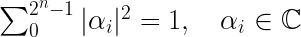
$\sum_{0}^{2^n-1} |\alpha_i|^2 = 1, \quad \alpha_i \in \mathbb{C}$

This tells us that a system of n classical bits can be fully described by n numbers, whereas a quantum system requires $2^n$ .

A quantum computer can hold exponentially more information, so it is so powerful.

Simulating a Quantum Computer

A double floating-point number can be represented on 8 bytes in classical memory. A 50 qubit system requires $2^{50} = 1,125,899,906,842,624$ bytes or 1 Petabytes. To give you some context, a supercomputer at NASA can have 2,016 nodes, with each node running 128GB of RAM for 252TB, a quarter of what’s required to run a 50-qubit simulator!

That by itself, however, does not explain the power of quantum computing. The truth is: an analog bit that can take any value from 0 to 1 can be said to represent a superposition of the two states.

So what makes quantum computers and qubits so special?

We can observe three major differences, at least, between a classical analog bit and a qubit: superposition, measurement, and entanglement.

3.3 Quantum Superposition

The first major difference between a qubit and a classical analog bit with a value of 0.5 is that the latter is just that. No matter how often you measure the analog bit, it will always show 0.5.

Now, consider a qubit in the following state:

$S_1 = \dfrac{1}{\sqrt2} (|0\rangle + |1\rangle)$

Each time we measure $S_1$ , we have a 50% chance of observing 0 or 1. We will never observe 0.5.

Taking Advantage of Superposition

The power of quantum computing lies in its ability to take advantage of superposition. If we use a qubit in a superposition of two states as input into our quantum computer and perform a single computation, we will process both states in a single shot.

On a classical machine, each input will have to be processed separately.

This may not seem like much for one qubit, but performance will scale significantly, although perhaps not exponentially, for practical reasons, which we will discuss in subsequent articles.

Is That All?

Superposition by itself does not tell the whole story. If you think about it, you will notice that running a measurement on a superposition of states will yield a random result for each measurement with probabilities defined by the amplitudes of each state. This is not very helpful. We need the system to produce the correct value. For this to happen, we need to use constructive interference, which we will discuss in greater detail in Part 2.

3.4 Quantum Measurements and Computation

The second difference between classical bits and qubits is the measurement exercise.

Thus, looking at the machine during the computation will invalidate the rest.

— Peter Shor – Polynomial-Time Algorithms for Prime Factorization and Discrete Logarithms on a Quantum Computer, 1996

Whenever we measure the value of a quantum system, we invalidate it. Scientists refer to a collapse of the wave function.

Going back to our analogy with the box and switch, we can state the following:

Before we open the box for the first time, the switch can be either ON, OFF, or both OF and OFF
Once the box is opened, the switch state will “collapse” to either an ON or an OFF state and remain in that state forever.

There is no distinction between the state of a bit before or after the measurement with classical bits.

3.5 Entanglement

Using the box and switch analogy, consider the following experiment.

Firstly, we make an identical set of boxes with one switch inside each.
Secondly, we move those boxes far apart so that they cannot influence each other when opened, even if they exchange photons running at the speed of light.
Finally, we ran a measurement on each box.

The result is as follows: The two boxes (or quantum systems) are said to be entangled if the outcome of the measurements is perfectly correlated.

For example, if we measure the first qubit and find it ON, we will notice that the second qubit will always yield OFF.

Einstein was unhappy with this phenomenon and referred to it as “spooky action on a distance” since it seemed to violate the Special Theory of Relativity. However, experiments have now unequivocally confirmed it.

3.5 Classical Gates

Inputs and outputs from classical computers are typically strings of bits which are then grouped into bytes to make up the different data types that a computer can process.

The way these bits are manipulated is as follows.

Classical computers pass these bytes, 2 bits at a time, into a sequence of logical, also known as Boolean, gates. Each gate will perform a Boolean operation such as AND, OR, XOR, or NOT.

The Universality of Logical Gates

Computer science tells us that these gates are universal. This means that a sequence of such gates, applied in a specific order, would allow us to compute any function we desire, such as addition, subtraction, or multiplication of two numbers.

For practical reasons, though, we only use a Negative AND or NAND gate. A combination of NAND gates allows us to emulate all the other logical gates, which, in turn, allows the implementation of every other function.

3.6 Computing with Quantum Gates

Quantum gates follow a similar logic. We have unitary gates that apply transformations to single qubits and binary gates that apply transformations to two bits simultaneously.

An example of a unitary gate is the Hadamard gate. It takes a $|0\rangle$ or a $|1\rangle$ , both pure (or eigen-) states, and transforms them into a superposition of the two states.

This is crucial as it allows us to design a multi-state, and therefore multi-input, qubit system that can be used to feed a quantum computer.

An equally important gate is the binary CNOT gate which allows us (in conjunction with the Hadamard gate) to entangle and disentangle two qubits.

The CNOT gate takes two inputs $|x\rangle$ and $|y\rangle$ and spits out two others. The first output is unchanged: $|x\rangle$ .

The second qubit will result from XORing the two input qubits: $|x\rangle \oplus |y\rangle$ .

3.7 Quantum Annealing

Another way that principles of quantum mechanics can be used to run quantum computations that can outperform classical computers is through quantum annealers.

These are different types of quantum computers that may not be as universal as those that use gates, which are the focus of this article.

Quantum annealers are designed to solve combinatorial optimization problems, the most popular of which is the Travelling Salesman Problem.

4. Quantum Solution to Deutsch’s Problem

Let’s practice some of these concepts and see what we get.

4.1 Problem Position

The best example of how quantum computing works is probably Deutsch’s algorithm.

The Deutsch–Jozsa algorithm is a deterministic quantum algorithm proposed by David Deutsch and Richard Jozsa in 1992 with improvements by Richard Cleve, Artur Ekert, Chiara Macchiavello, and Michele Mosca in 1998. Although of little current practical use, it is one of the first examples of a quantum algorithm that is exponentially faster than any possible deterministic classical algorithm.

— Wikipedia

The problem that Deutsch proposed was as follows: with a single evaluation, determine whether a unitary function $f(x)$ is constant or balanced.

By definition, a constant function always returns a 0 or a 1, regardless of the value of x. The only two examples of constant functions we know of are $f(x) = 0$ and $f(x) = 1$ .

Also, by definition, a balanced function will return a value. The only two examples we can find are the Identity $f(x) = x$ and the Negation $f(x) = \bar{x}$ functions.

Typically, you need to evaluate $f(x)$ at least twice to find the answer, as running the function only once does not provide us with enough information. On quantum computers, though, the Deutsch algorithm allows us to do that with a single evaluation.

4.2 Deutsch-Josza Algorithm

The following diagram describes Deutsch’s algorithm applied to a quantum computer.

deutsch algorithm quantum computing — Deutsch’s algorithm

We have already encountered the Hadamard gate (H), the measurement gate, and the CNOT gate, but we have not discussed the f-CNOT gate.

The f-CNOT gate is just a modified version of the CNOT gate where x is replaced with f(x) before the XOR operation occurs.

$f\textendash CNOT |xy\rangle = |f(x) \oplus y\rangle$

It’s nothing more than applying f(x) to the input before CNOT.

4.2.1 Step 1: Preparing the Inputs

The first step is fairly simple. In it, we prepare two qubits in the ON state.

$\Psi_{step 1} = |11\rangle$

4.2.2 Step 2: Creating Quantum Superposition

In step two, we apply a Hadamard gate on each qubit to transform its state into a superposition of ON and OFF. This allows us to obtain an input variable with all four possible combinations of qubit states:

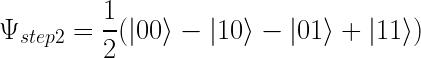
$\Psi_{step 2} = \dfrac{1}{2} ( |00\rangle - |10\rangle - |01\rangle + |11\rangle)$

This is where the magic happens. The system in this superposition state will allow us to perform all four evaluations simultaneously.

4.2.3 Step 3: Evaluating f(x)

In this step, we look at the operation outcome f-CNOT will perform on the input from Step 2. The result is as follows:

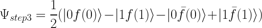
$\Psi_{step 3} = \dfrac{1}{2} ( |0f(0)\rangle - |1f(1)\rangle - |0\bar {f}(0)\rangle + |1 \bar{f}(1)\rangle)$

Look at the first term $|0f(0)\rangle$ . This is the outcome of the transformation of $|00\rangle$ .

Because the first qubit is 0, the CNOT gate will not flip the other one. Notice how that is not the case in the second term. Indeed the 0 has been flipped to 1.

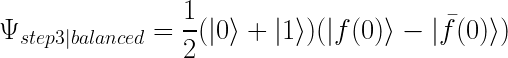
We must consider two cases to understand how this will help us solve our problem. The first is when $f(x)$ is constant, and the other is when $f(x)$ is balanced.

With a little bit of elementary algebra, we can arrive at the two situations:

If $f(x)$ is constant, we obtain:

$\Psi_{step 3|constant} = \dfrac{1}{2} ( |0\rangle - |1\rangle)(|f(0)\rangle - |\bar{f}(0)\rangle)$

On the other hand, if $f(x)$ is balanced, we get:

$\Psi_{step 3|balanced} = \dfrac{1}{2} ( |0\rangle + |1\rangle)(|f(0)\rangle - |\bar{f}(0)\rangle)$

But how does that help us determine the nature of $f(x)$ ? The key to solving this problem lies in the first factor of both equations:

$\dfrac{1}{2} ( |0\rangle + |1\rangle)$

And:

$\dfrac{1}{2} ( |0\rangle - |1\rangle)$

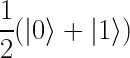
4.2.4 Step 4: Finding the Result

Taking a closer look at these two equations, you will probably recognize them as the outcomes of the Hadamard gate for inputs $|0\rangle$ and $|1\rangle$ although differing by a factor of $\dfrac{1}{\sqrt{2}}$ .

We know that the Hadamard gate if applied to the two inputs in superposition, will allow us to recover the original inputs $|0\rangle$ and $|1\rangle$ . And this is exactly what we will do.

The function is balanced if the outcome is $|0\rangle$ . Otherwise, it’s constant.

4.3 What Does Deutsch’s Algorithm Tell Us About Quantum Computing

We can see Deutsch’s problem and solution as an example of those exponentially more difficult to solve on classical computers but take only a few steps to resolve on quantum computers.

It also tells us that some effort needs to be made to reformulate the problem to allow us to take advantage of superposition or any other quantum phenomenon.

5. Further Reading

Richard Feynman. QED: The Strange Theory of Light and Matter (book review)

Operational Excellence

Organisational Culture

Organisational Processes

Project Delivery

Soft Skills for Engineers

Computer Science and Engineering

Quick Links